| token | frequency | |
|---|---|---|
| 0 | Sijnde | 657 |
| 1 | nog | 2192 |
| 2 | voorders | 185 |
| 3 | gecompareert | 61 |
| 4 | jacobus | 564 |
Standardisation and Orthographic Variation in Late Modern Dutch Witness Depositions
Using Transformers to Detect Spelling Variation
Sara Budts, Yoshi Malaise, Rik Vosters
Step 1: Preprocess the Corpus
Clean all the text files and generate a nice wordlist with their frequencies of the target language.
Get rid of:
- transcription remarks
- spurious line endings
- punctuation
- numbers
- Other languages in the text
- …
Extract the Tokens and Vocabulary
nlp = spacy.load("nl_core_news_md")

def tokenize(text):
    return [token.text.lower() for token in nlp(text)]

def get_vocab(corpus):
    vocab = []
    for text in corpus:
        vocab.extend(text)
    return vocab

tokens = []
for text in all_texts:
    tokens.append(tokenize(text))
vocab = get_vocab(tokens)
counter = collections.Counter(vocab)
Step 2: Create vector embeddings
Create vector embeddings of all words with a minimal frequency of 2
Load the frequency wordlist from the first chapter
Filter words that appear less than twice
Calculate vector embeddings for remaining words
What are vector embeddings?
Intermezzo: Vector Embeddings
Computers love numbers!
They are easy to work with, can be used in calculations and are less open to interpretation.
Embeddings are a technique to approximately represent a concept by an ordered list of numbers (The vector!).
In theory the size of the vector and the range/meaning of the numbers can be anything, as long as we apply it conistently to all of the elements we want to work with.
Intermezzo: Vector Embeddings
Word Embeddings
If we want to create Word embeddings could manually try to come up with a list of attributes that we fill in for each word in our vocabulary, but this would be very tedious and time consuming.
Luckily, these days powerful computers can learn meaningful representations by exposing them to a large set of textual data to train on. We no longer know exactly what each number in the vector represents, but we do not really need to know as long as we can use the model to get our desired results.
Intermezzo: Vector Embeddings
Transformers
Being able to represent words as vectors is a great first step, however remember embeddings are ways to represent concepts. Not every concept can easily beexpressed by one word.
For example: “The president’s wife”, “my oldest brother”, “almost satisfied”
To work with these concepts we need a way to create a sort of “combined vector” that not only looks into the embedding of the current word but also takes into consideration the influence of the embeddings of the surrounding words to construct a vector.
A common architecture for this is the Transformer Model, based on which pre-trained systems have been created such as BERT.
Intermezzo: Vector Embeddings
Tokens
Up until now we simplified the working by pretending that we always work on complete words.
But what would happen if we encounter a new word that we never encountered during the initial training? If there is no matching Word embedding it cannot be used to influence the final representation. So instead of only relying on full words, we also create vectors for frequently occuring word pieces (suffixes, prefixes, commonly occuring parts). If the word is not recognised, we split the word in the largest recognised parts called tokens.
It is exactly this property of the model that we will exploit to find spelling variations. Many historical words will not be recognised as-is but as a sequence of wordpieces.
kuikentje procureur prockueur
We will use a modified version of BERT, called GysBERT, to construct an embedding for each of the words in our dataset.
# Extract the embeddings from the encoding layer of GysBERT
batch_size = 100
first_batch = True
for i in range(0,len(vocab)+batch_size,batch_size):
    print(i)
    input = tokenizer(vocab[i:min(len(vocab)-1,i+batch_size)],return_tensors="pt",padding=True)
    output = model(**input)
    embeddings_batch = output["last_hidden_state"][:,0,:].detach().numpy()
    if first_batch:
        embeddings = embeddings_batch
        first_batch = False
    else:
embeddings = np.concatenate([embeddings,embeddings_batch])Step 3:
For each word, find the closest word by looking at the distance between the embeddings.
Find closest words
We construct a table with all the words as both the rows and the columns
| word 1 | word 2 | word 3 | word 4 | word 5 | ... | word 1001 | word 1002 | word 1003 | word 1004 | word 1005 | ||
|---|---|---|---|---|---|---|---|---|---|---|---|---|
| 0 | word 1 | - | - | - | - | - | - | - | - | - | - | - |
| 1 | word 2 | - | - | - | - | - | - | - | - | - | - | - |
| 2 | word 3 | - | - | - | - | - | - | - | - | - | - | - |
| 3 | word 4 | - | - | - | - | - | - | - | - | - | - | - |
| 4 | word 5 | - | - | - | - | - | - | - | - | - | - | - |
Find closest words
We fill this table with the cosine difference between two words (w1 and w2) at the coordinates [w1,w2].
The smaller the angle between the two vectors, the more similar they are to each other. Of course in reality, we are not simply doing this in a 2D grid, but in a many dimensional space.
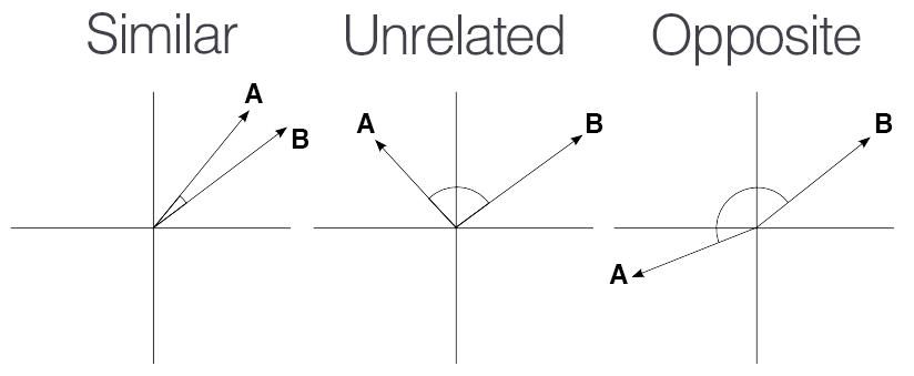
cosine distance
Find closest words
Once this table is created we can perform a lookup to find the nearest neighbor of each word in our wordlist (this will be the one with the lowest cosine distance).
Based on this we write the output file bootstrap_annotations_from_encoder.csv.
Find closest words
| token | frequency | nearest neighbor | distance | label | same | |
|---|---|---|---|---|---|---|
| 0 | heeft | 15081 | heeft | 0 | 1 | |
| 1 | voor | 5030 | vóór | 0 | 0 | |
| 2 | la | 1844 | là | 0 | 0 | |
| 3 | die | 7528 | dië | 0 | 0 | |
| 4 | syn | 548 | sÿn | 0 | 0 |
In this table we can find for each word in the vocabulary how frequent it appears, its nearest neighbor, the distance between the two embeddings, a label which we will leave empty for now, and a value indicating whether the embedding has the same written text.
Find closest words
In future steps, this file will serve as the basis for some fine tuning. To achieve this we will need to manually annotate (parts of) this file.
Step 4: Annotate the generated pairs
Annotate the generated pairs
Sort the file by ascending differences
Label wordpairs based on their relationship (e.g., same word, diacritic difference only, …), decide which pairs to keep for future training and whether or not they are treated as spelling variation.
Sort the table based on the value in the distance field.
Remove all the pairs with the same word (not variants as they are identical).
Put the pairs with the lowest value first (e.g. these are most likely to be variants)
Annotate the generated pair
| token | frequency | nearest neighbor | distance | label | same | |
|---|---|---|---|---|---|---|
| 1 | voor | 5030 | vóór | 0 | 0 | |
| 2 | la | 1844 | là | 0 | 0 | |
| 3 | die | 7528 | dië | 0 | 0 | |
| 4 | syn | 548 | sÿn | 0 | 0 |
Annotate the generated pair
Next, label the wordpairs using the following conventions:
| label | meaning | keep? | variants? |
|---|---|---|---|
| S | Same Word | X | X |
| FR | French | X | X |
| D | Diacritic Difference Only | V | V |
| ORT | Orthographic Difference | V | V |
| MORF-ORT | Orthographic or Morphological Variant | V | V |
| SEM | Semantically Related but not Morphologically | V | X |
| UNC | Unclear | V | X |
Step 5: Train a New Classifier
Use the labeled data from the previous step as the training data to create a new binary classifier that predicts given a pair of words whether they are spelling variants.
Architecture Recap:
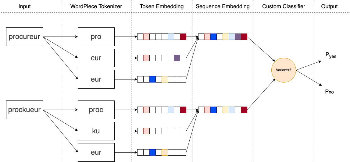
Remember, the goal is to create a system that can predict whether 2 words are spelling variants.
Architecture Recap:
To achieve this we leverage the existing WordPiece tokenizer found in GysBERT to split these words into frequently occuring wordpieces, for which Token Embeddings exist.
Architecture Recap:
GysBERT is then used to combine all the embeddings for a word (a word can consist of any arbitrary number of tokens) into 1 fixed length vector for each word.
Architecture Recap:
Since we now have a fixed size for each wordpair (e.g., 2 times the length of the sequence vector) we can design and train a binary classifier that given 2 Sequence Embeddings can predict how confident it is that the wordpair is (\(p_{yes}\)) or isn’t (\(p_{no}\)) a spelling variant.
Training the classifier
It is this classifier of the final step that we will train.
For this we follow a predetermined workflow:
- Use a k-fold cross validation approach to tune hyperparameters on the labeled data.
- Use best result to predict labels for all unseen data
- Take a sample of 1000 wordpairs stratified by the confidence of the prediction (e.g. 0-10%, 10-20%, …)
- Manually correct the labels of the sample and add it to the labeled data
- Accept current results, or go back to step with the the new labeled data as additional trainingdata.
- in our implementations we included 3 additional cycles.
Step 6: Manually Label Candidate Pairs
We use the best performing model from step 5 to predict the chances that each possible wordpair is a spelling variation.
If a pair has more than 5% predicted chance to be a variation collect it in a new dataset and label whether it is in fact a variation.
The Cut-off
The 5% cut-off is chosen by hand.
We feel this is a relatively good balance between the amount of labelling work while still being certain we can catch most spelling variants.
A lower cut-off will lead to more potential pairs being detected which will need to be labeled (a cut-off of 0 would mean manually label every pair in the entire corpus).
A higher cut-off will result in less pairs being flagged (we only ask for validation on pairs the computer is already pretty sure of) but this of course comes with the risk that many variants go undetected.
Step 7: Cluster the Variants
Go through all the variants in the generated file and assign them in clusters according to transitivity. If A is a spelling variant of B and B is one of C, then A and C are variants of each other too.
Example
The following table:
| Word 1 | Word 2 |
|---|---|
| gesaemelyck | gesaementlijck |
| gesaementlyck | gesaemelyck |
| inschelijcx | inschelÿcx |
| inschelijcx | insgelijcx |
Example
Results in these clusters:
Where words in each cluster are expected to be variants of each other.
B-TXT